Word Vectors in the Eighteenth Century, Episode 2: Methods
0. Disclaimer
This post is a write-up of what I’ve learned about what word vectors are and how they work. I often feel it’s not until I try to explain something that I realize the ways in which I don’t quite understand it. That was the case here, and what follows is a wrestling of myself into a (partial) understanding of the subject.
For a more comprehensive and capable introduction to word vectors, please see Ben Schmidt’s “Vector Space Models for the Digital Humanities” (25 Oct 2015). Schmidt’s post is introductory, practical (with instructions for how to use word vectors in R), and theoretical. And Teddy Roland has recently published an IPython notebook detailing how to get started with word2vec using Python’s gensim package.
What follows here is another explanation: a conceptual one, that tries to understand the basic logic behind word vectors. It’s still perhaps redundant; but it was useful to me, and may be also useful to others. As a final note, if anyone reading this notices anything inaccurate, please let me know!
1. The original word vector: the document-term matrix
In order to understand what’s new about the kind of vector representation in a word embedding model, I think it’s helpful to remember the ways in which we’ve already been using word vectors in DH.
A classic form of data representation in DH is a document-term matrix.[0. Although document-term matrix might be the most paradigmatic case, a term-term matrix-based on counts of term collocation in a “window” of N words long-is also standard, and produces a similar kind of word vector.]
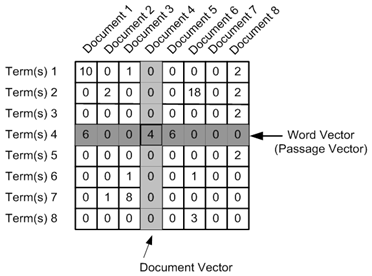
Figure 1: Example of a document-term matrix
As the figure shows, a document-term matrix represents a given term as a word vector: a vector of its number of occurrences in each document:
Term(1) = (10, 0, 1, 0, 0, 0, 0, 2)
Term(2) = (0, 2, 0, 0, 0, 18, 0, 2)
...
Here, “vector” has the meaning it does in the programming world: as an array, that is, a list of numbers.
But many DH studies have also taught us to imagine each “column” of these numbers as representing a unique dimension in space. Each term then occupies a different spatial position in an N-dimensional space, where N is the number of documents. We can then find similar terms to a given Term(X) by finding words close to it spatially. Spatial proximity between any two points A and B can be measured in different ways:
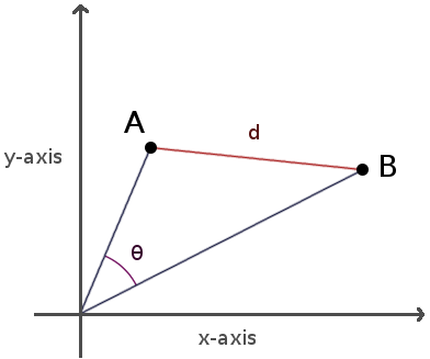
Figure 2. Euclidean distance (d) vs. Cosine distance (ϴ)
For instance, we could measure the Euclidean distance (using the distance formula) between two points A and B; or we could measure the cosine of the angle formed between the two vectors A and B drawn from the origin point. Here, the word “vector” is taking on its geometric definition: a geometric object with a direction connecting an initial point P1 (the origin) to a terminal point P2 (a given term’s position in the document-space).
Problems with the original word vector
All of this is great, has produced incredible work, and will continue to do so. But there are (often) two problems with representing words as vectors of their counts in documents. First, there are often too many documents, or, too many dimensions. At the very least, this can present computer processing challenges, but it can also present statistical problems related to the the Curse of Dimensionality-the phenomenon by which adding more dimensions actually makes the matrix more sparse, more full of zero-values, since each new document will score “0” on many, maybe most, of the included terms. The louder data-noise in this sparse matrix makes it less tractable for statistical analysis, rendering measures of statistical significance less robust and its representation of semantic relationships less accurate.
The other problem is that defining the similarity of two words as their similarity of occurrences across documents is not exactly the most contextually sensitive way we can imagine representing word similarity.[0. Term-term matrices based on word collocation might get around this problem, but not the previous one (about matrix size). And since the document-term matrix seems more frequently used in DH, this second problem still seems worth bearing in mind in general.] For instance, one of the most frequent words of the eighteenth century is “virtue”; and we can imagine that the word “virtuous” occurs similarly often when measured across the same documents. But “virtue” is a noun, an abstract noun, often personified, often held out as a singular idealized entity; whereas “virtuous” is an adjective, and usually applied to particular persons or behaviors. We can always hope that these differences between the two words would register, somehow, in their differences of frequency across the documents. But what would be preferable is a model sensitive enough to encode both their semantic similarities (as words of the same root, words of moral discourse) and their semantic differences (noun vs. adjective, universal vs. particular, etc).
2. The new word vector: word embedding models
This is where word embedding models (WEMs) come in: they offer a powerful and elegant solution to these two problems. Rather than represent a word as a vector of its counts in documents, where the number of dimensions can be statistically unwieldy, a word embedding model embeds a word in a lower-dimensional space in ways that end up better representing the semantic and syntactic relationships between words. In these models, words are represented as vectors along a few hundred artificial dimensions-that is, dimensions that don’t correspond to documents or other real textual contexts.
At this point, however, word embedding models differ by algorithm and software package. One scientific paper I found distinguishes between “context-counting” and “context-predicting” word embedding models.[0. Baroni, Dinu, Kruszewski: “Don’t count, predict! A systematic comparison of context-counting vs. context-predicting semantic vectors” (Proceedings of Association for Computational Linguistics, 2004)] The new GloVe package by the Stanford NLP group, released in 2014, and already the primary competitor to Google’s word2vec, is a count-based model. It first constructs a giant matrix of every word as the rows, and every word again as the columns. Then, churning through slices of text 10 words long, the matrix is continuously updated with the number of times word X and word Y were seen together in a collocation window. This giant matrix of word-to-word collocation counts, is then, somehow, according to math I don’t understand, “factorized” down to a reasonable numble of dimensions, while still representing most of the variance, or information, in the original giant matrix. Count-based models, working via dimensionality reduction, have been developing for a long time in the computational linguistics community. DH studies have often used them, as well: PCA, LSA, even topic modeling, are all ultimately forms of count-based dimensionality reduction.
The other type of word-embedding model is prediction-based, and developed out of the machine learning community. These models’ capacity to render semantic relationships between words was initially perceived as an interesting byproduct of their capacity to solve “deep [machine] learning” tasks. The implementation that has generated so much buzz, Google’s word2vec, published in 2013, uses a particular kind of machine learning algorithm called an artificial neural network. Artificial neural networks, inspired by biological neural networks and cognitive science research, can actually learn, or predict, things. Given thousands of objects as inputs and being continually asked to guess what they are, the neural network gradually reconfigures a “hidden layer” of neurons such that it’s best able to represent the “input layer” (features of the object) well enough to predict the “output layer” (what the object is).
But that’s a description of neural networks in general. In a neural network word embedding, the “hidden layer” of neurons is the word embedding; the 50-500 neurons are the 50-500 dimensions along which words are represented as vectors.[0. Which, incidentally, is why I can’t help but feel that neural network word embeddings would be fascinating material for anyone working at the intersection of cognitive science and DH.] Each word is represented as a vector, not of counts in documents, but of quantified de/activations in each neuron:
Term(1) = (0.2, -0.6, 0.9, ...)
Term(2) = (-0.5, 0.1, 0.3, ...)
When “displayed” Term(1), it’s as if Neuron(1) fires +0.2, Neuron(2) fires -0.6, and so on.
The model is initialized with completely random vectors for each word: a scrambled, cyberpunk version of Locke’s tabula rasa. It then gradually reprograms and improves these vectors in order to better perform a given task. For example, one way word2vec can learn word vectors is to be presented with huge numbers of “valid” 5-grams, like “cat sat on the mat”, as well as a huge number of “invalid” 5-grams that have been randomly “broken” by a word substitution, like “cat sat song the mat.” The model then has to decide if the 5-gram is valid or invalid. It does so by continually reprogramming its vectors such that, over time, the “broken” words are, in comparison to their four valid fellows, outliers to the valid words’ neighborhood within the vector space.
Problems with word embedding models
The actual math behind this process is beyond me-which brings me to what seems to be the major weakness of word embedding models. Even for those who do understand the math behind WEMs, exactly why or how they produce the dimensions they do seems to be impenetrable. At the end of the day, it’s a black box.
But a useful black box.[0. The same defense could be made of the varying degrees of black-boxness of most other dominant DH methods: topic modeling and text classification, for example. Although the mathematics, statistics, and logic are well understood, at some finer grain of explanatory detail the light goes out. As with word embedding models, I don’t think this is a problem, necessarily, so long as this explanatory blindspot is noticed and somewhat understood.] WEMs provide a spatial representation of word similarity that is statistically robust and has been demonstrated to provide state-of-the-art accuracy in a wide range of NLP tasks.
However, even more interesting, to me, than their usefulness, is their elegance…
3. So, how does queen = king + woman - man?
So how is a vector space model able to express an analogical relationship between words? Let’s work out by hand the canonical example: Man is to Woman as King is to Queen, or in other “words”, V(Queen) = V(King) + V(Woman) - V(Man).
Before we do, drawing on my high school algebra, let’s subtract V(King) from both sides of this equation, so we can rewrite it equivalently as V(Queen) - V(King) = V(Woman) - V(Man). Let’s look at both of these vector subtractions separately, V(Woman) - V(Man) and V(Queen) - V(King), first semantically and then mathematically.
Semantic subtractions
V(Woman) - V(Man)
Let’s first look at V(Woman) - V(Man), on the right side of the equation, V(Queen) - V(King) = V(Woman) - V(Man). This is an example of a vector subtraction. Mathematically, it works by subtracting the score for V(Man) from the score for V(Woman) along each dimension of the vector space (i.e. the 50-500 dimensions of neuron de/activations in the neural network). But we can also think of this subtraction semantically. What are some of the semantic aspects of the words “Woman” and “Man” that we would expect to be expressed somewhere in the model?
| Woman | Human being | Adult | Female | Noun | ? |
|---|---|---|---|---|---|
| Man | Human being | Adult | Male | Noun | ? |
| Woman - Man | 0 | 0 | Female - Male | 0 | ? |
Table 1. Semantic aspects of the words “Woman” and “Man”, and the resulting semantic subtraction of Woman-Man.
In other words, “Woman” is a noun for an adult, female human being. “Man” is a noun for an adult, male human being. If we subtract these semantics of “Man” from the semantics of “Woman”, then their shared semantic aspects are eliminated, and we’re only left with a single semantic difference: of their genders, “female” and “male.” Thus, what is left is only a particular semantic axis of difference: “gender”, as conceived as a spectrum, or vector, from male-ness to female-ness.
V(Queen) - V(King)
Now let’s look at V(Queen) - V(King), on the left side of the equation, V(Queen) - V(King) = V(Woman) - V(Man). Again, mathematically, this works by subtracting their scores along each dimension. But semantically, how would this subtraction work?
| Queen | Human being | Monarch | Female | Noun | ? |
|---|---|---|---|---|---|
| King | Human being | Monarch | Male | Noun | ? |
| Queen - King | 0 | 0 | Female - Male | 0 | ? |
Table 2. Semantic aspects of the words “Queen” and “King”, and the resulting semantic subtraction of Queen-King.
Queens and kings are semantically different from women and men: they’re monarchs, and not necessarily adults. But since they’re both monarchs, the semantic subtraction of King from Queen again leaves only one semantic axis of difference: gender. Thus to subtract King from Queen produces the exact same semantic difference that’s produced by subtracting Man from Woman. In mathematical terms: V(Queen) - V(King) = V(Woman) - V(Man). Recall that this equation is equivalent to V(Queen) = V(King) + V(Woman) - V(Man), the original equation. So, semantically, this is Q.E.D., what was to be demonstrated.
Vector subtractions
But we can also demonstrate that V(Queen) = V(King) + V(Woman) - V(Man) mathematically rather than semantically by doing the math and drawing the vectors. So, let’s pretend for a moment that our model has only two dimensions. Of course, in practice there will be 50-500 dimensions, not 2, so all of this becomes more complicated, but it remains essentially the same process. Here are the (made-up) vectors, then, for the three words, “woman”, “man”, “king”.
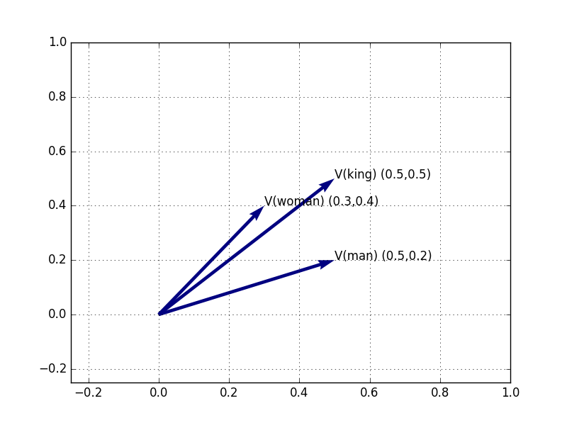
Figure 3: V(Woman), V(Man), and V(King) in 2-dimensional space
Again, let’s break this down one operation at a time. First, let’s compute V(Woman)-V(Man). We already know the vector positions for both V(Woman) and V(Man), so we can work this out mathematically by hand:
V(Woman) - V(Man)
= (0.3, 0.4)
- (0.5, 0.2)
= (-0.2, 0.2)
These are therefore the coordinates for a new vector, expressing the direction toward V(Woman) from V(Man). We can label this vector V(Woman-Man) and plot it in the same way:
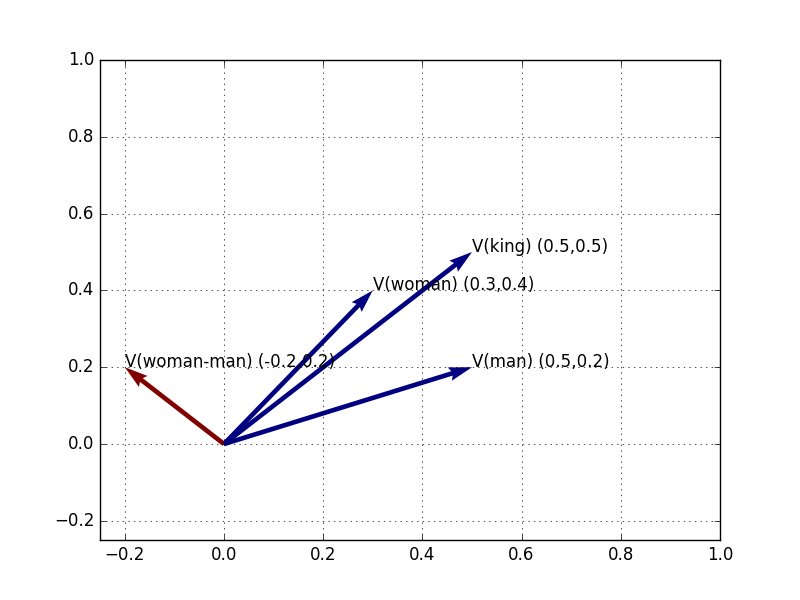
Figure 4: V(Woman), V(Man), V(King), and V(Woman-Man)
We can make sure this is right by re-drawing this same vector, V(Woman-Man), not from the origin point, but from V(Man):
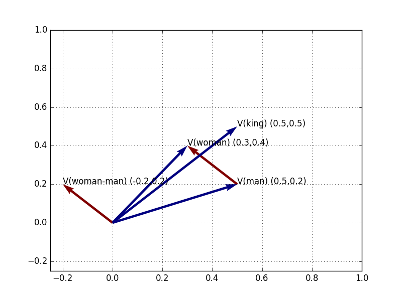
Figure 5: V(Woman), V(Man), V(King); and V(Woman-Man), plotted from origin and from V(Man)
Starting at V(Man), to move along the semantic axis of gender, V(Woman-Man)-in the semantic direction toward V(Woman) and away from V(Man)-brings us back to V(Woman). This is tautological: it can be expressed mathematically as the sum of the gender difference V(Woman-Man) and V(Man), which simply reverses the procedure we did previously:
V(Woman-Man) + V(Man)
= V(Woman) - V(Man) + V(Man)
= V(Woman)

V(Woman-Man) + V(Man)
= (-0.2, 0.2)
+ (0.5, 0.2)
= (0.3, 0.4)
= V(Woman)
But, non-tautologically, we can do the same thing from the different departure point of V(King). We want to locate the vector pointing to this point:
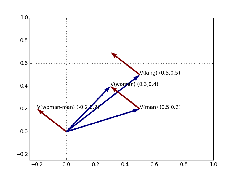
Figure 6: V(Woman), V(Man), V(King); and V(Woman-Man), plotted from origin, from V(Man), and from V(King)
We can find that vector by adding the gender difference of V(Woman-Man) to V(King):
V(Woman-Man) + V(King)
= (-0.2, 0.2)
+ (0.5, 0.5)
= (0.3, 0.7)
Drawing a line to this vector, we discover that the closest nearby vector is indeed, V(Queen)!
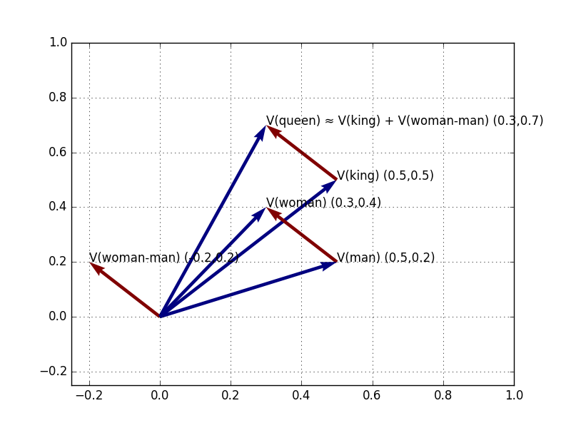
Figure 7: V(Woman), V(Man), V(King); V(Woman-Man), plotted from origin, from V(Man), and from V(King); and V(king+woman-man), which is closest to V(Queen)
Why is this? It’s not magic: it’s because, as we saw in the “semantic subtraction” section above, the vector of semantic difference (gender) between Woman and Man is the same vector of difference (gender) between Queen and King. This is why to move along V(Woman-Man), from V(King), gets us to V(Queen). Or in other words, V(Queen) = V(King) + V(Woman) - V(Man). Q.E.D.!
That’s all for now. For some initial experiments distant-reading eighteenth-century semantics, stay tuned for the next episode of “Word Vectors in the Eighteenth Century”…
-1. Appendix
In this appendix I want to address a couple of technical questions for word2vec: optimal skipgram size and minimum corpus size.
Optimal skipgram size
One of the most important parameters in training a word embedding model is the size of the “skip-gram” to train on. Default word2vec settings use skip-grams of 5 words long; GloVe uses 10 words. Word on the word embedding street is that smaller skip-gram sizes (especially of 2 words long) amplify syntactic relationships and dampen semantic relationships, while larger skip-gram sizes do the reverse.
It’s hard to know exactly how to determine the optimal skip-gram size, but I ran a couple of experiments on models trained on the same corpus (ECCO-TCP) with different sizes. Here’s the 25 most similar words to “virtue” for each model:
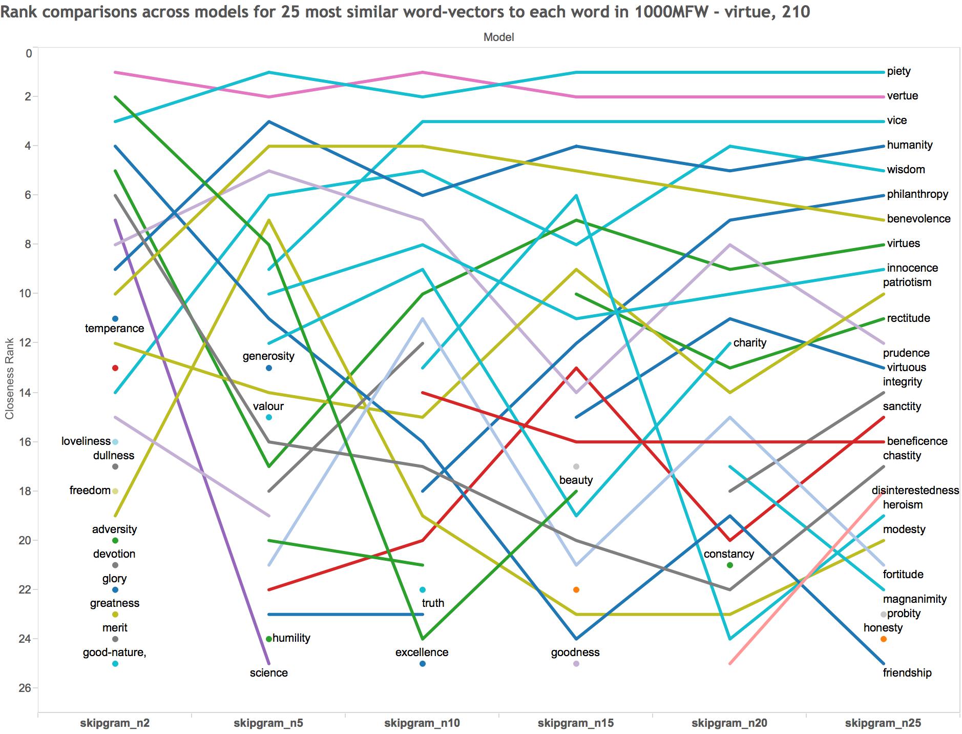
Figure 8: The 25 most siilar words to “virtue”, in word2vec models of ECCO-TCP using skip-grams of 2, 5, 10, 15, 20, and 25 words long.
The second most similar word to “virtue” in the model trained on skip-grams of only two words long is “beauty” (the dark green line). “Beauty” subsequently declines through the models trained on longer skip-grams. Insofar as two-word skip-grams are picking up on syntactic similarities, this makes sense to me: both “beauty” and “virtue” may govern similar verbs and adjectives. But although virtue was considered beautiful in the period, “beauty” is not exactly what I would think of as the second most semantically similar word to “virtue.” What I would expect-words like “vice”, “humanity”, “wisdom”, etc.-appear in the models trained on skip-grams of >2 words.
Another approach to the question of optimal skip-gram size would be to evaluate the “accuracy” of each model according to a set of analogy tests compiled by Google:
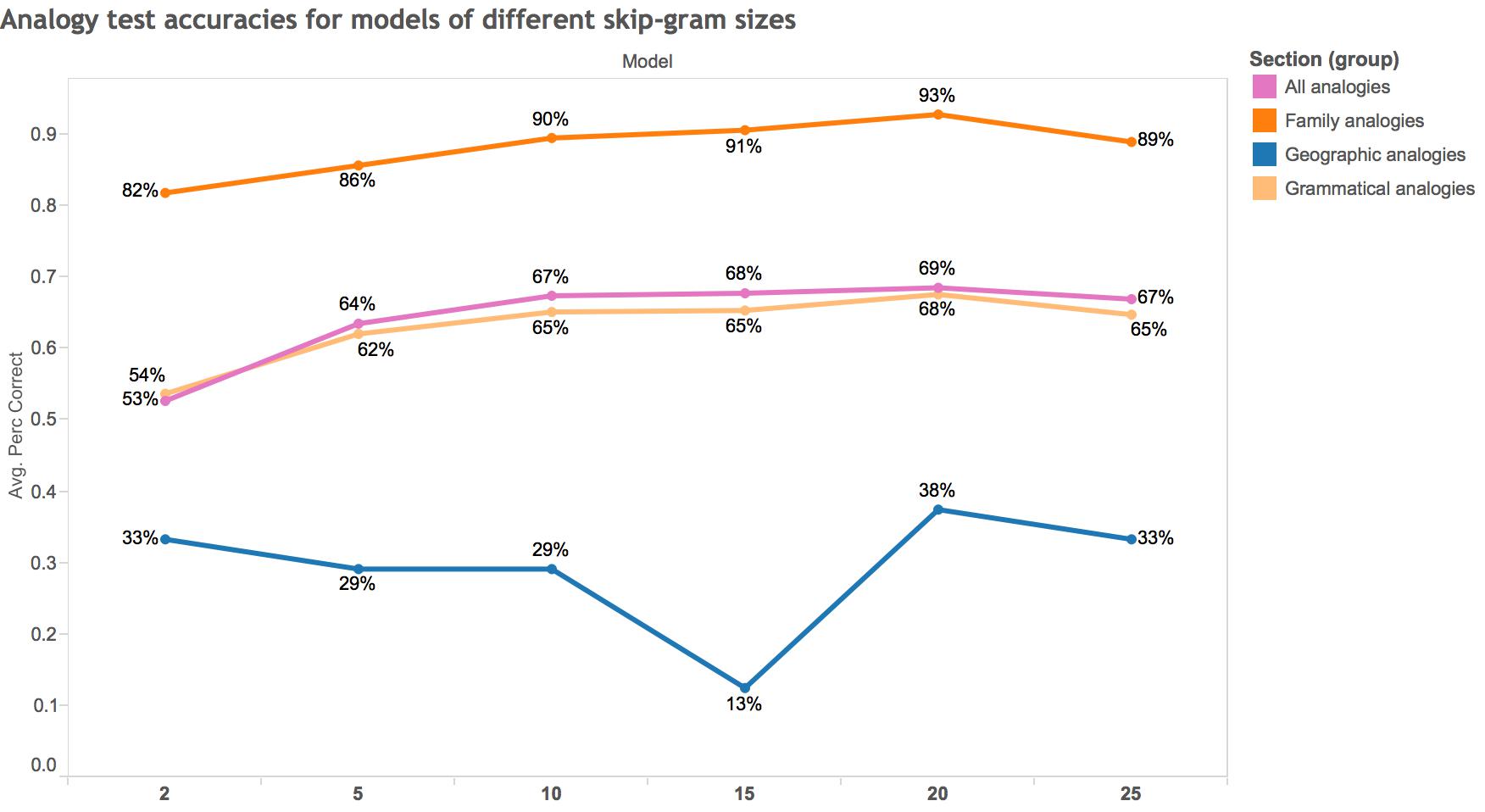
Figure 9: Analogy test accuracies for models of different skip-gram sizes, broken down by type of analogy. Questions come from analogies compiled by Google. Analogies are only considered if all four words of the analogy are in the most frequent 5,000 words of the corpus. A “baseline” accuracy could be 74.26%, what the total accuracy is for a Google-trained model on Google News (1 billion words) using 300 vectors and (I believe) five-word skip-grams.
What’s striking to me is that, according to these analogy tests, the two-word skip-gram model performs worse on almost every metric-all but the geographic analogies (mostly capital to country), which I expect are not as coherently presented in ECCO-TCP as they are in the Google News corpus on which word2vec was initially trained. The “hump” in the data seems to be skip-grams of ten words long: after that point, the gain in accuracy is minimal.
To sum up, I personally come away from these experiments thinking that a ten-word skip-gram model might actually be optimal-at least for this corpus and for the kinds of semantic questions I want to ask of it. Ten-word skip-grams seem to produce intuitive semantic similarities and good accuracy on the analogy tests. Since I uploaded a five-word skip-gram model of ECCO-TCP last time, I’ve uploaded here a ten-word skip-gram model of ECCO-TCP. Let me know if you’re interested in any other models. [Incidentally, I’m working now on building a word2vec model of all of ECCO Part I (154k documents); I’ll hopefully be uploading that soon.]
Minimum corpus size
Another important technical question concerns how large a corpus needs to be to yield an accurate word2vec model. I approached this question similarly, and measured how accurately models of different corpus sizes (all samples from ECCO-TCP) perform on analogy tests.
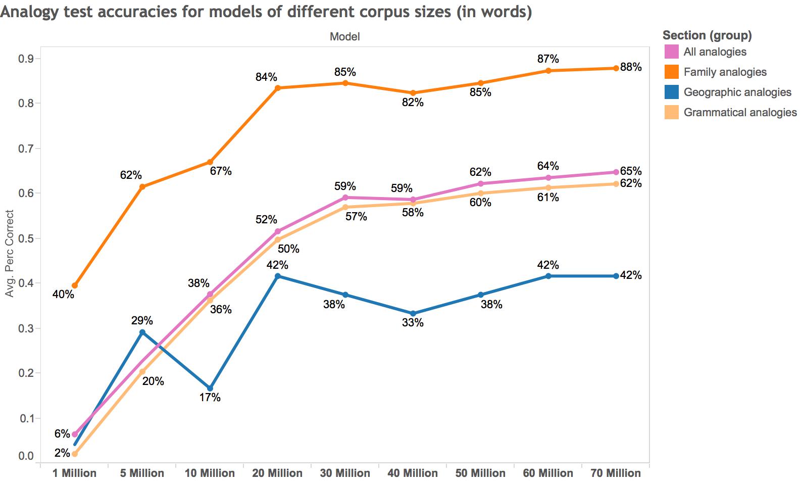
Figure 10: Analogy test accuracies for models of different corpus sizes (measured in words), broken down by type of analogy. The differently-sized corpora are derived from differently-sized samples of all 5-word skip-grams in ECCO-TCP. Questions come from analogies compiled by Google. Analogies are only considered if all four words of the analogy are in the most frequent 5,000 words of the corpus. A “baseline” accuracy could be 74.26%, what the total accuracy is for a Google-trained model on Google News (1 billion words) using 300 vectors and (I believe) five-word skip-grams.
I’m not exactly sure how to interpret this, but it seems to me that around 30 million is a “hump” past which accuracy gains are more minimal. That said, the difference between 30 and 70 million words is an absolute difference of 6% accuracy gain, which seems meaningful to me. Given that a “baseline” accuracy (based on a massive Google News corpus) for “All analogies” might be 74%, I imagine that accuracy increases with corpus size more and more gradually toward that limit.
In sum it seems like a ten-word skip-gram model, on a corpus of 30 million words or more, might be a good rule of thumb for thinking about corpus size and model parameters when building your own word2vec model.